GUI tutorial

How to use the GUI of findmycells

Launching the GUI:

The GUI of findmycells is intended to be used by users with limited python programming expertise. Therefore, launching the GUI is kept as simple as possible. All you need to do is run the following two lines of code in a Jupyter Notebook!

from findmycells.interfaces import launch_gui
launch_gui()

Note

This tutorial uses the findmycells sample dataset for the most part. If you want to recreate the same steps on your local machine, feel free to download the sample dataset (including images, ROI files, and a trained model ensemble), which is hosted on Zenodo. Checkout the “Download the full sample dataset” section below for how and where you can download it.

The individual steps of creating and running a findmycells project:

1) Start a project:

You can start a project either in an completely empty directory (findmycells will then automatically create all subdirectories that are required), or with an already existing subdirectory structure. Here, we will start completely from scratch in an empty directory:

2) Add all your data

Now, please grab some snacks, as the following piece of information is quite important, but unfortunately also quite a bit to read - bare with us!

Before we can continue with our project in the GUI, we first have to add all our data to the project. This needs to be done by adding the image data in a very specific structure to the “microscopy_images” subdirectory. This structure consists of three subdirectory levels that correspond to different metadata information of your experiment:

1st level: main group IDs
2nd level: subgroup IDs
3rd level: subject IDs

Simply start by creating one folder for each of your main experimental groups (for instance “wildtype” and “transgenic”, not limited to any specific number) inside of the “microscopy_images” subdirectory. Now, into each of these main group folders, you have to add a folder for each experimental subgroup within this main group. This can be for instance different timepoints (e.g. “week_01” and “week_04”; again, not limited to any number). However, this may of course not be applicable for all experimental designs. Sometimes, you may simply not have any subgroups within your main groups. Nevertheless, this subdirectory level is required. In such a case, simply add a single directory and feel free to give it any name (note, that also in the sample dataset, there will only be a single subgroup ID folder). Finally, in each of these subgroup folders, please create a folder for each experimental subject from which you acquired the image data (unique IDs required!). Into each of these subject ID folders, you can now add all corresponding image files. Phew - done!

Please have a look a the following tree to see an example of how this could look like. Note, that there is no specific number of images required in each of the subject folders, that the images in the different subject folders can even have the same names, and that subject IDs have to be unique. Obviously, subject folders places inside the “wildtypes” main groub directory, are consequently considered to belong to this main group (and likewise to the respective subgroup).

project_root_dir:
│ 
└── microscopy_images:
    │ 
    ├── wildtypes:
    │   ├── week_01:
    │   │   ├── mouse_01:
    │   │   │   └── image_01.png
    │   │   │   └── image_02.png
    │   │   └── mouse_02:
    │   │       └── image_01.png
    │   │       └── image_02.png
    │   │       └── image_04.png
    │   └── week_04:
    │       └── mouse_03:
    │           └── image_08.png
    │ 
    └── transgenics:
        ├── week_01:
        │   ├── mouse_04:
        │   │   └── image_01.png
        │   │   └── image_05.png
        │   └── mouse_05:
        │       └── image_01.png
        │       └── image_02.png
        └── week_04:
            ├── mouse_06:
            │   └── image_01.png
            │   └── image_02.png
            │   └── image_03.png
            └── mouse_07:
                └── image_01.png
                └── image_08.png

Note

You will always be able to update the files that are associated with your project. So, for instance, you can already start with an intial subset of your image data and keep on adding files later on to the same project, if you aquire more data along the way!

You also have the chance to investigate only specific regions of your images. This can speed up computation times and reduce memory load, but might also add more specificity to the insights you can derive from your image analyses. In findmycells, this can be done by providing a ROI file associated to each microscopy image. To do this, simply copy the exact same directory structure you just created for your images and copy-paste it into the “rois_to_analyze” subdirectory. Now replace each image file with a ROI file (see below for how you can & should create these), while that the ROI-file has the exact same filename as the corresponding image. For instance, for the image with the filepath:

project_root_dir/microscopy_images/wildtypes/week_01/mouse_01/image_01.png

The ROI file should be named & placed like this:

project_root_dir/rois_to_analyze/wildtypes/week_01/mouse_01/image_01.zip

Currently, only ROI-Sets created with ImageJ are fully supported (and highly recommended). Please have a look at the following gif, to see how you can easily create such a ROI-Set:

Important

To ensure full functionality of findmycells it is highly recommended to provide a ROI-Set (.zip file!) created with ImageJ for each of your images, in which you renamed all individual ROIs accordingly (see gif above). This is true even if you only want to analyze a single area in an image, as ImageJ does not support to rename the ROI to anything different than the filename. However, since the filenames are used to match ROI-files with the corresponding images - this causes inconsistencies. Thus, even if you only want to analyze a single area in an image, simply add a second ROI (can for instance be small and placed anywhere inside the actual ROI) and rename it to something that does not match with your actual area IDs (like “not_a_real_area”).

Tip

This structure may be complicated to grasp at the beginning. Therefore, please feel free to check out our sample dataset and compare the directories, filenames, images, and corresponding ROI files. Even if you don’t want to download the full dataset, you can also just browse through it in our GitHub repository here.

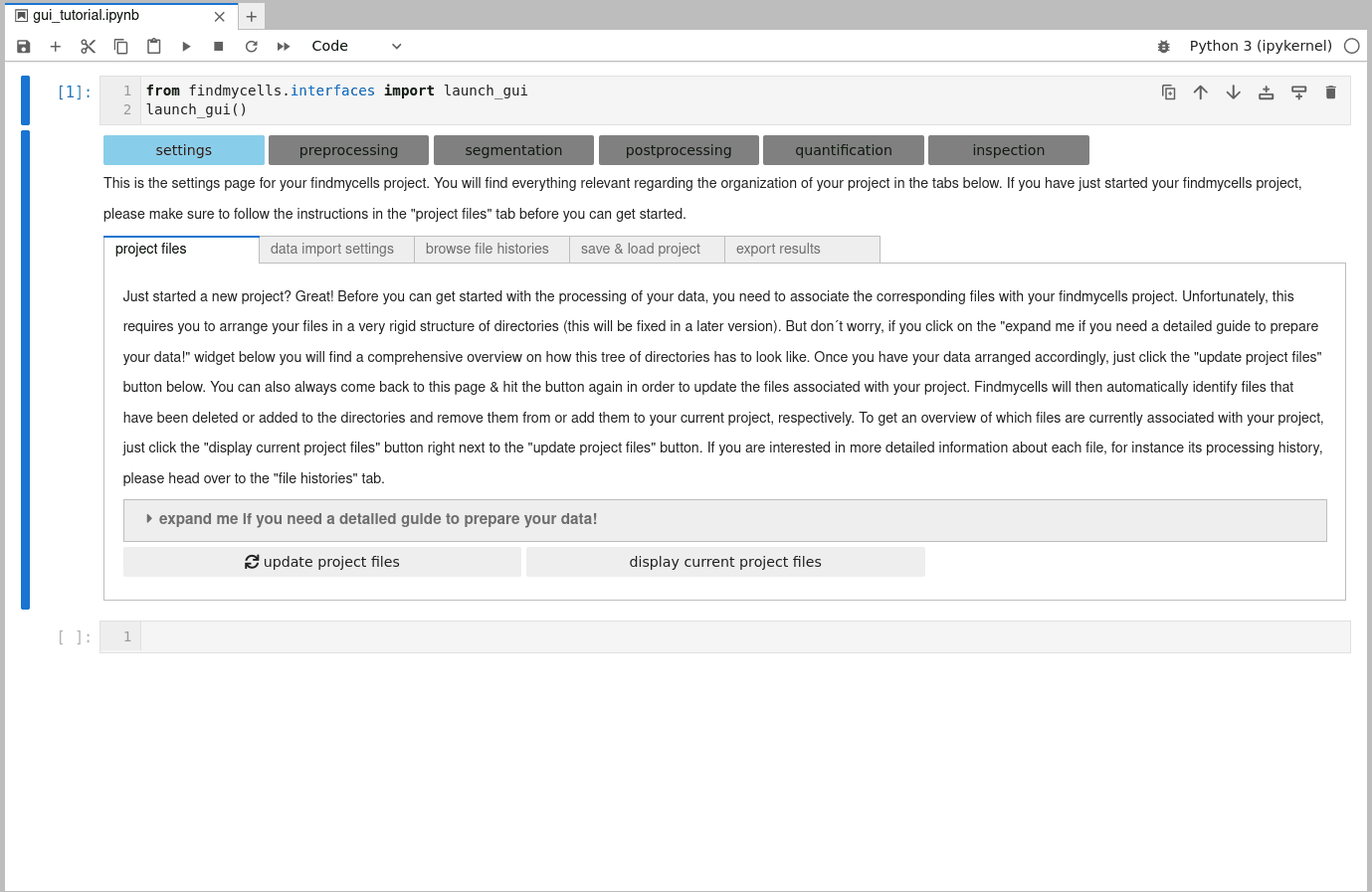
3) Import all metadata information into your project

findmycells creates and maintaines a database for you that keeps track of all your files & how (and when) you processed them. Once you placed all image files (and, optionally, all associated ROI files) in the corresponding subdirectory trees, your good to go & can use the “update project files” button. findmycells will now confirm that your file structure is indeed as expected and will then infer all the relevant metadata information. Note: the actual image or ROI data will not be loaded into memory at this moment. If successfull, you should now see a table that lists the detected files with the inferred metadata information:

4) Specifying how to import image & ROI files:

Next, you have the option to specify how the image data and the ROI files shall be imported in the “data import settings” tab, still on the settings page. Since this time it’s really about how these data will be loaded into memory, it may make sense to limit everything right away only to a certain color channel or only to a few specific planes, in case you’re working with a z-stack. However, this is entirely up to you & you can also play around a bit and try different options until you found the perfect settings for you. Please remember to click on the “confirm settings” button for both, the Microscopy images and the ROI files.

Tip

To preview whether the selected data import settings meet your expectations, you can simply continue with the preprocessing of your images (see the next section below) on a limited number of files and then confirm that the created preprocessed images in the “preprocessed_images” subdirectory match your expectations. If not, simply return to this widget, adjust some of the values & re-run the preprocessing (remember to check “overwrite previously processed files”).

5) Preprocessing of your data:

Now you finally made it to the core part of findmycells - the processing of your image data. All of the following processing pages (i.e. “preprocessing”, “segmentation”, “postprocessing”, and “quantification”) will look very similar to each other and, therefore, also work very similarly. Thus, let’s discuss the preprocessing page in great details, and then go through the other pages a littler quicker.

a) Select a processing method:

For all processing steps, you will be prompted to select one (or several) of the available processing methods. These resemble different options how your data gets processed. On each processing page, you will have a so-called accordion widget that you can expand by clicking on it to reveal its content. In the expanded accordion, you will see a dropdown menu that lists all available processing methods for the respective processing step. For preprocessing, these include for instance “Convert into 8-bit format”, “Adjust brightness and contrast”, or “Maximum intensity projection”. Once you select a option, a more detailed description of this method will appear below, alongside some additional customization options (if applicable). To include a processing method in your project, select it in the dropdown menu, adjust the customizable settings, and then click the “confirm selection & export configurations” button. This will then cause the accordion to collapse again and to create a second accordion. The first accordion will now display the name of the processing method you selected. You can always click on it to expand it’s content again & use the “remove method” button to remove it from the list of processing methods again, in case you changed your mind. Feel free to add as many processing methods as you like, but please be aware that they will be executed in the order that you selected them in (i.e. in which they are displayed to you - top to bottom).

Important

Currently, findmycells evolves entirely arround deepflash2 and cellpose as segmentation tools. While this may change in future versions, it is strongly recommended to run the “Convert into 8-bit format” as last preprocessing method, to ensure full compatibility with these tools.

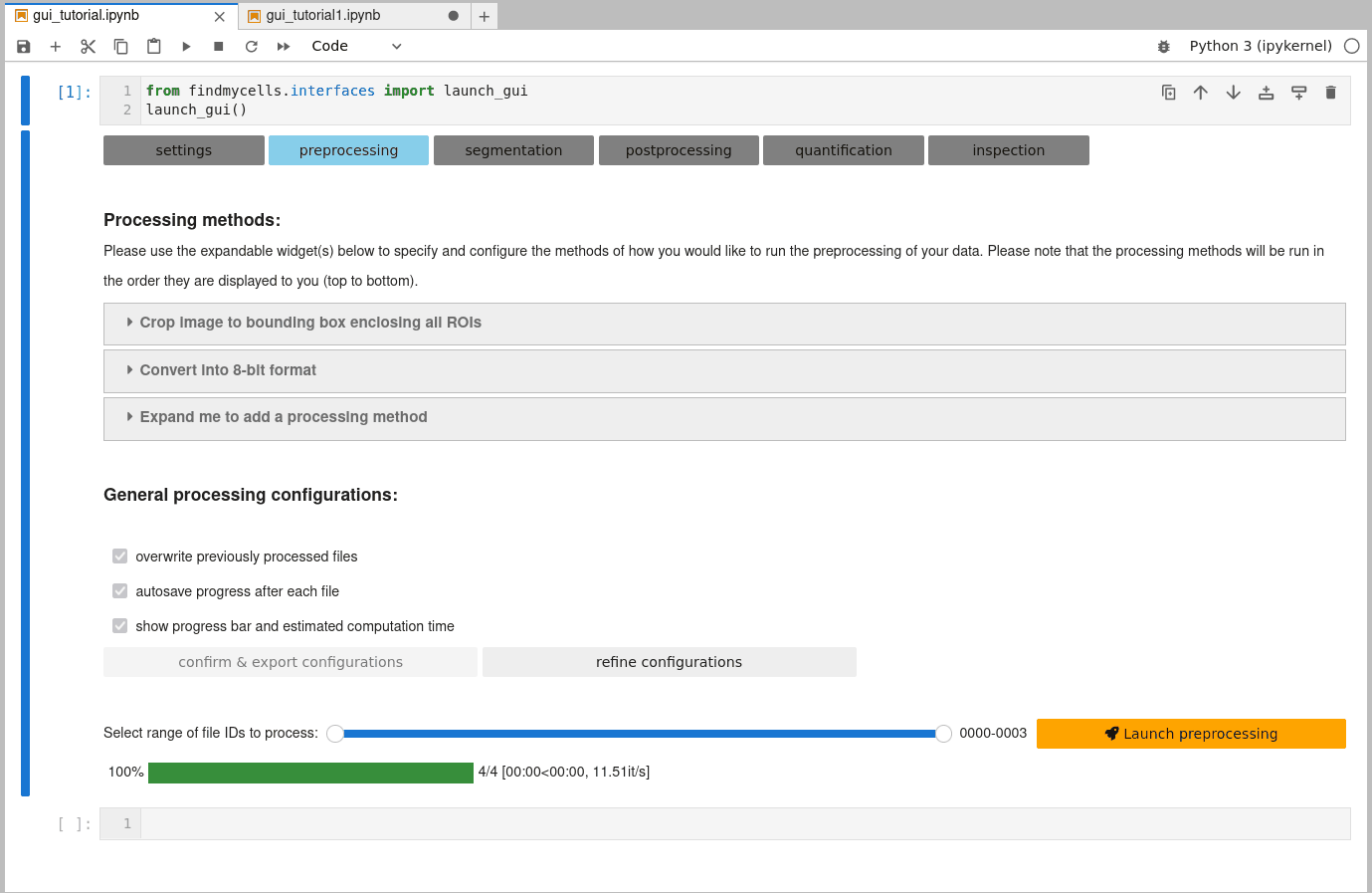
b) Customize general processing settings:

Once you are happy with the selection of processing methods, you need to confirm some general processing configurations. These include, for instance whether findmycells should try to save the progress of your project as soon & wherever possible (autosave progress after each file), or whether files that you may have processed earlier already shall be overwritten or skipped. Please click the “confirm & export configurations” button to fix your current selection. In case you’d like to change anything again - use the “refine configurations” button to make the widgets interactive again.

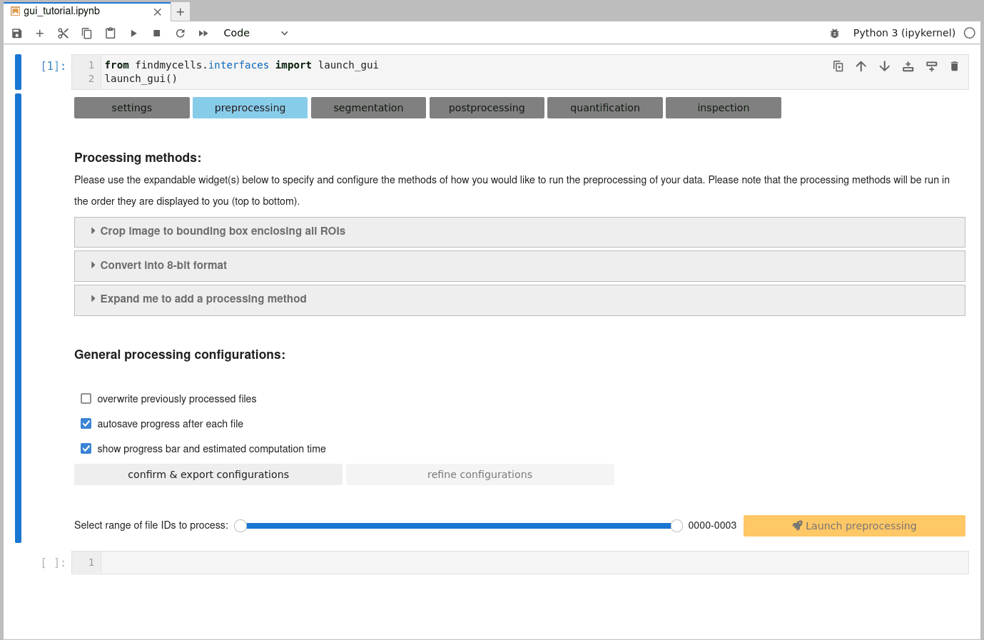
c) Select files to process & launch processing step:

The last thing that remains to do is to specify the range of file IDs you’d like to process. By default, all files will be selected. Feel free to had back to the “project files” tab on the “settings” page, to take a look at the overview table that shows what file ID refers to which of your original files. When you’re ready - it’s finally time to hit that “launch processing” button!

Tip

You will find the preprocessed images in the “preprocessed_images” subdirectory. We highly recommend to confirm that they all look as expected, before you continue with the following, more time consuming processing steps.

6) Segmentation of your data:

You will need to specify the path to the directory of where the corresponding trained models of the deepflash2 model ensemble can be found. Remember, they have to be compatible with the version 0.1.7 of deepflash2. Feel free to store them in your project root directory, to have them always clearly associated with this project - or to load them from a directory outside of your project root. For now, you only have the options to create semantic segmentations only (by using deepflash2 alone), or to create instance segmentations derived from these semantic segmentations (by using cellpose after deepflash2).

Important

If you want to create instance segmentations, you will need to either finish semantic segmentations of all files first, or to specify a diameter that cellpose is supposed to use. Why? Well, cellpose tries to separate touching features based on flow gradients that rely on an estimated mean diameter of these features. This diameter can be estimated by cellpose (recommended - just leave the “diameter” slider at 0), or be provided by you. However, if you want cellpose to compute it, it will require all semantic segmentations first, to make the estimate as accurate as possible.

7) Postprocessing:

Once you managed to get all segmentations, you’re almost done! Next up, you can run some post-processing on the segmentation masks, for instance applying exclusion criteria to filter for clearly biological relevant & meaningful features.

Note

In case you are working with a 3D (2.5D) dataset and created instance segmentations, you also have the option to re-construct the features in 3D by running the “Reconstruct features in 3D” method. This method also needs to be run before applying exclusion criteria.

If you don’t run this strategy, the instance labels will most likely not be matching across the individual planes.

8) Quantification:

Not much to say here - runs the quantification of the detected features in your postprocessed segmentation masks per area.

9) Inspection:

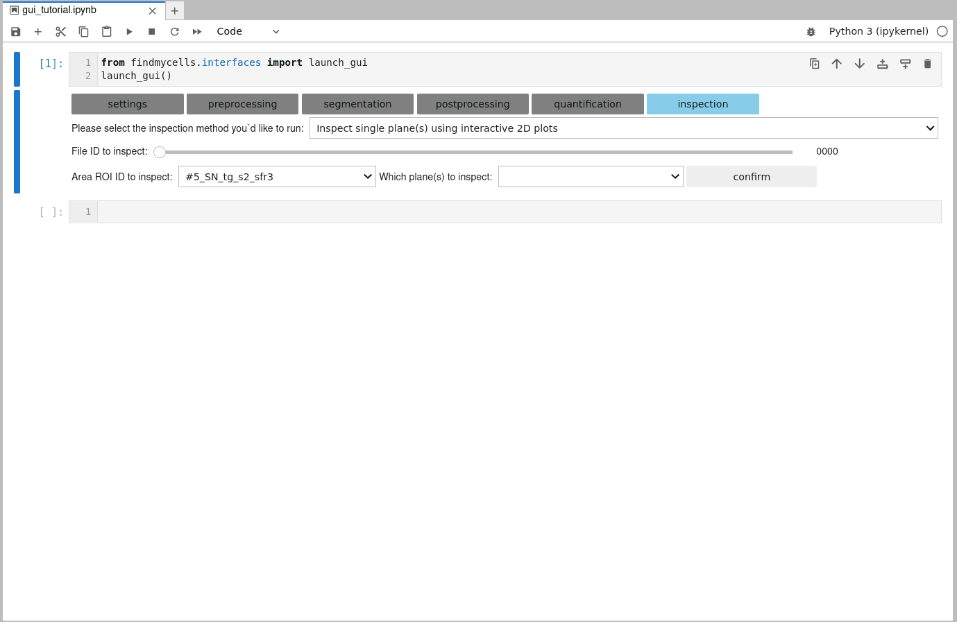
The GUI of findmycells also comes with some in-built functions that allow you to create interactive plots to take a very close look at how the final, postprocessed and ultimately quantified segmentations look like. For this, head over to the “inspection” page & chose one of two inspection methods: 2D or 3D. You can also run 3D inspection on a 2D dataset and 2D inspection, on a 3D dataset - but usually 2D inspection on 2D data, and 3D inspection of 3D data, makes most sense.

After selecting a file ID, the area ID, and which plane(s) should be included in the plot, you will be prompted with some additional configuration options. Since the images used in findmycells are usually quite large, the inspection plot will be focused only on a particular section of the image. You can use the customization widgets to specify how big this section should be, and where it should be centered. Among these widgets, you will find three features that support you in your selection process. You can either open an interactive plot that allows you to zoom in and and out of the image-mask-overlay, while displaying the exact pixel coordinate of where your cursor is pointing in the bottom right corner. Alternatively, you can also select one of the unique IDs of the detected features in this image from the dropdown menu. Upon selection, the coordinates of this features centroid will be computed and printed to the right of the dropdown menu. In case of a 3D dataset in which you run the “Reconstruct features in 3D” postprocessing method, you might also have some feature IDs listed in the “multi-match-traceback” dropdown menu. These features were found to partially overlap also with other features and, hence, might be of particular interest to take a closer look at.

The following gif shows you the inspection of the 2D data in the cfos_fmc_test_project sample dataset:

Tip

You can also save the current view of the interactive plots that open in a separate window, if you’d like to! Simply use the little save icon in the bottom left corner.

While processing of 3D (2.5D) datasets works just as demonstrated for the 2D sample dataset shown above, let’s have a look at a more interesting 3D inspection plot below:

10) Detailed file history:

As mentioned before, findmycells keeps a detailed record of your files and how you processed them. To take a look at this information, head over to the “settings” page, click the “browse file history” tab & then select a file ID you’d like to know more about:

11) Save & load projects:

Of course findmycells supports saving & loading of your current project status. This can be done again on the “settings” page, in the “save & load project” tab. The two files that store all relevant information of your project (.dbase and .configs) will be saved by default in your project root directory. Please do not move these files anywhere else! You can delete older versions of the files, though (as determined from the date as prefix).

12) Export quantification results:

As soon as any quantification results are computed by your findmycells project, you can use the “export results” tab on the settings page to export these results either as .csv or as .xlsx spreadsheets. The quantification results will be separated by area IDs into different different files & findmycells will also add some additional metadata that might come in handy for your subsequent statistical analyses.

Tip

The output format of the quantification results is designed to match the expected input format of the python tool stats_n_plots, which was also developed by the Defense-Circuits-Lab and represents - just as findmycells - an interactive jupyter-widget GUI that helps you perform statistical analyses and create appealing plots of your data in no time!

Advanced functionalities:

Well, let’s face it. Most likely, you will run into an error and something will stop working / not work as intended. In these cases, it may be beneficial to have the findmycells project object (an instance of the API class) available as variable in your jupyter notebook, rather than just as GUI-widget. Therefore, we recommend that users who are in general familiar with objects and basic python syntax, use the following lines to launch the GUI:

from findmycells.interfaces import GUI

gui = GUI()
gui.displayed_widget

This allows you to access everything stored in the project also via the gui variable. For instance, after initializing a project and updating the project files, you can use:

gui.api.database.file_infos

to see what files are currently associated with your project. Or:

gui.api.database.file_histories

to browse through the individual FileHistory objects of each file ID.

Download the full sample dataset:

If you are interested in downloading our full sample dataset, including images, ROI-files, and a trained model ensemble, you can do so either manually from our Zenodo repository, or by using the following lines of code:

from findmycells.utils import download_sample_data
from pathlib import Path

destination_dir = Path('/please/provide/a/path/to/an/empty/directory/on/your/local/machine/here')
# If you wish to run the download, simply remove the hashtag at the beginning of the following line:
#download_sample_data(destination_dir_path = destination_dir)